UW-Eau Claire Geography 335: GIS 1 Blog: 2016

Sunday, May 15, 2016

GIS 335 Final Project

Goals and Background: For our final term projects in GIS I, we had to develop a geospatial question and find the answer to it by obtaining the necessary data and analyzing it in ArcMap properly. For my term project, I looked at ideal locations for turkey hunting in Rice County. I based this on the criteria of habitats where turkeys would ideally be found, where the most urbanized areas of the county are, and parameters of needing to be off of the road in order to shoot. Ideal turkey habitats are in areas near water sources, as well as any areas that have grassy fields or lots of trees. My intended audience was anyone looking to either purchase land to hunt on, as well as anyone traveling to the area looking for a place to hunt turkeys. This project is important because it can help people make more educated decisions on where they will go to find turkeys for hunting.

Methods:
I started this project by downloading my data from the Minnesota Geospatial Commons and ensuring it was all in the same projection. In ArcMap, I selected Rice County from the MN Counties layer and created a new layer of it. I then clipped all of my other vector data down from the entire state of Minnesota to be just in the parameters of Rice County. In order to get the landcover raster to be clipped down to the area that I needed I had to go through a very different process than just simply using the clip tool. I had to use the reclassify tool to incorporate binary functions to give me results of only the specific types of landcover classes that meet turkey habitat requirements. Then I used the raster clip tool to clip that down to be just that of Rice County. To convert this raster into vector data, I used the raster to polygon tool. I then used the select by attributes tool to extract the specific landcover types that ended up being all combined into one. Regardless, this still gave me the landcover information I needed so I could proceed. I placed a 2 mile buffer around urban areas because there aren’t any good hunting areas in the heart of a city. The only exceptions I included were areas that are wildlife refuges specifically there for hunting purposes. I placed a buffer of 15 yards around all of the roads to ensure laws as well as proper hunting safety measures are accounted for. I put a 1 mile buffer around all open water in Rice County because ideal habitats for turkeys are near an easy water source. I intersected the water buffer with the turkey habitat landcover layer and then erased the street buffer from that. After that I erased the urban buffer from the previous layer in order to eliminate all of the parameters that would not be good for turkey habitats. Finally, I merged that layer with the wildlife refuge layer because, even though the wildlife refuges fall within the urban buffer zones, they are an exception due to the nature of their existence. I created a new data frame and put the layer of all the Minnesota counties into it and selected Rice County in order to create a locational reference map. I then switched over to layout mode and created a map document with both of these. The results of this can be seen in Figure 2 below.

Figure 1: This is the data flow model of all the tools and layers I used for my project.

Results:

I found that there are a lot of areas in Rice County that meet the ideal turkey habitat requirements. The ideal hunting areas seem to be most heavily distributed toward the western half of the county, especially around some of those bigger lakes. Most of the urban areas don’t even meet the requirements for turkey habitats, but it is still important to not hunt in those areas unless under special circumstances to ensure people’s safety. The southeastern quadrant of the county has very minimal areas that would be good for hunting turkeys.

Figure 2: My final map of turkey hunting locations in Rice County, as well as a locational reference map.

Sources:

Minnesota Geospatial Commons. (n.d.). Retrieved May 10, 2016, from https://gisdata.mn.gov/

Recognizing Wild Turkey Habitat. (n.d.). Retrieved May 08, 2016, from http://www.wildernesscollege.com/wild-turkey-habitat.html

Wednesday, May 4, 2016

Geography 335 Lab 5

Goals and Background: The main goals of this lab were to gain experience using a variety of vector geoprocessing tools to create a map of a geospatial problem, to learn the basic use of Python scripting to run various tools, and to gain experience creating digital data workflow models.

Methods: For part 1, I started off by downloading the data I needed and using ArcCatalog create a feature class out of the XY data provided to me in an excel document. I then made sure they were all in the proper and same coordinate systems and changed them if need be. I then added all of the bear_management_area feature classes to a blank map in ArcMap and symbolized the landcover layer based on minor types. I intersected the bear locations with the landcover layer to figure out what the ideal landcover types for bears are. I then buffered the streams by 500 meters, and intersected that resulting layer with the previous ideal bear landcover layer to determine their overall ideal habitat locations. I made sure to run a dissolve function to ensure that there wouldn't be any internal boundaries that could skew further analysis of the data. I then intersected the study_area layer with the dnr_mgmt area to narrow the DNR land to be just in the area of study. Then I intersected that area with the suitable bear habitats area to select all suitable bear habitats that also fall into DNR land. Then I symbolized the landcover layer to be by major types, selected all urban areas, and created a layer of those. I created a 5km buffer around the urban areas, and then used the erase feature, combining that layer with the suitable dnr area layer to give me a layer of only the dnr areas that are the proper distance away from urban land. I then renamed the layers and made a map that showed these areas. It can be seen in the section below.

Digital Data Workflow Model for Part 1

Part 2 was my first attempt at learning Python scripting to find the ideal location for a new resort. I added the Wisconsin cities, lakes, interstates, and counties layers to a blank map in ArcMap. Then I used python coding to create a 10 mile buffer around the major cities.

I then wanted to find lakes that had an area greater than 5 square miles:

I then wanted to exclude any lakes that didn't meet all of my criteria, so I used the clip tool:

Then I created a map of these results, as seen in the next section.

Digital Data Workflow Model for Part 2-1

Next, I wanted to examine pollution levels around interstates. To do this, I used a multiple ring buffer analysis tool around the interstates layer through python coding:

Results:

Map 1, showing bear management solutions for the DNR

This is the first map from part 2. It shows eligible lakes for tourist resorts in Wisconsin.

This is the 2nd map from part 2. It shows the pollution zone levels around the interstates of Wisconsin.

Sources:

Esri - GIS Mapping Software, Solutions, Services, Map Apps, and Data. (n.d.). Retrieved April 28, 2016, from http://www.esri.com/

Michigan Department of Natural Resources. (n.d.). Retrieved May 04, 2016, from http://www.michigan.gov/dnr

Price, M.H. (2015). Mastering ArcGIS. Dubuque, IA: McGraw-Hill Higher Ed.

Wilson, C. (2012). A comprehensive Lake features for Wisconsin.

Tuesday, March 29, 2016

GIS 1: Lab 4

Goals and Background: The main purpose of this lab was for me to practice using Boolean expressions, operators, and parenthesis to develop multiple criteria SQL queries to extract and isolate components of data from a database. It was also intended to give me experience using both spatial queries and attribute queries as well as map the results of the data I isolated.

Methods: The first part of this lab dealt with queries of the entire United States. I started out by opening ArcMap and adding the "counties" layer from the USA geodatabase. For the first question, I had to write a multiple criteria query that will return counties with a population between 3,000 and 4,000 people in 2010, as well as all counties in 2010 that had a population density of at least 1,000 persons per square mile. To do this, I opened the select by attributes window and entered the following query:

This gave me a result of 194 counties selected. I right clicked on the "counties" layer and chose to create a new layer from the selection so I could analyze them further on their own. I opened the attribute table of this new layer, summarized the state name field, and added that table to the map so I could see it. I concluded that 35 states were included among these counties. I was also able to see the mean and standard deviation. I then made a map of the selected counties, as seen below. To do this, I switched to layout view and added a title, scale, north arrow, and legend.

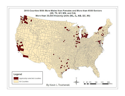
For the second question I searched for counties in the states of Wisconsin, Texas, New York, Minnesota, and California where the male population is greater than the female population, as well as the number of seniors is over 6500. To do this, I used the select attributes window and entered the following:

This gave me the criteria I was looking for, only in the states I specified. I then created a layer of these resulting counties, and summarized a table of the state name features so I could see how many counties with these attributes were in each state. I then created a map of these counties using the same steps as above.

The third question had me modify the second query to also include all seniors in Maryland, Nebraska, Washington, Illinois, DC, and Michigan who live in counties with more than 30,000 housing units. The attribute query I used for this is as follows:

For this query, the parenthesis were very important to group the proper portions of the query together and to ensure that their order of operations would be followed to give me the results I wanted. I created a new layer of these features and then mapped them accordingly in the layout view mode.

Part 2 of this lab involved me creating queries to analyze and isolate data in the state of Wisconsin. I first had to download the data from a private UWEC source and unzip it. I added the counties, lakes, and cities shapefiles to a blank ArcMap document for question 4. This question had me develop a query that isolated cities in the state of Wisconsin that had populations of between 15,000 and 20,000 people, more females than males, the area of the city is at least 5 square miles on land, and are within 2 miles of a lake. This involved me using two types of queries: an attribute query, and a location query. For the attribute query, I entered:

This got the cities narrowed down to everything except the 2 miles from a lake requirement. For that, I had to use the select by location window. I entered the following into that window:

This gave me the rest of what I needed. I made sure it was set to select from other currently selected features to ensure that it would continue to meet all of the other criteria that I previously searched for in the select by attributes window. This narrowed it down to 3 cities, which I created a separate layer for, and then mapped them in the layout view window while also adding the major roads shapefile to give more context to the map.

The final question involved me mapping and finding the total length of several major rivers in Wisconsin. To do this, I added the rivers shapefile to the Wisconsin map and used the following attribute query to select the rivers I wanted to isolate:

I created a separate layer of these rivers and looked at the statistics of the "PMILES" field. I needed to find the combined length of all of these rivers, but the sum statistic was far to big of a number to be realistic. I realized that the data was actually in meters and converted it separately to be the miles measurement that I needed. Then I created a map of all of these rivers with major roads and lakes as a reference. I added labels to the rivers to make the map more aesthetically pleasing and useful.

Results: