GIS 1: Lab 4

Goals and Background: The main purpose of this lab was for me to practice using Boolean expressions, operators, and parenthesis to develop multiple criteria SQL queries to extract and isolate components of data from a database. It was also intended to give me experience using both spatial queries and attribute queries as well as map the results of the data I isolated.

Methods: The first part of this lab dealt with queries of the entire United States. I started out by opening ArcMap and adding the "counties" layer from the USA geodatabase. For the first question, I had to write a multiple criteria query that will return counties with a population between 3,000 and 4,000 people in 2010, as well as all counties in 2010 that had a population density of at least 1,000 persons per square mile.  To do this, I opened the select by attributes window and entered the following query:



This gave me a result of 194 counties selected.  I right clicked on the "counties" layer and chose to create a new layer from the selection so I could analyze them further on their own.  I opened the attribute table of this new layer, summarized the state name field, and added that table to the map so I could see it.  I concluded that 35 states were included among these counties.  I was also able to see the mean and standard deviation.  I then made a map of the selected counties, as seen below.  To do this, I switched to layout view and added a title, scale, north arrow, and legend.

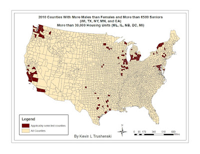
For the second question I searched for counties in the states of Wisconsin, Texas, New York, Minnesota, and California where the male population is greater than the female population, as well as the number of seniors is over 6500. To do this, I used the select attributes window and entered the following:

This gave me the criteria I was looking for, only in the states I specified. I then created a layer of these resulting counties, and summarized a table of the state name features so I could see how many counties with these attributes were in each state.  I then created a map of these counties using the same steps as above.

The third question had me modify the second query to also include all seniors in Maryland, Nebraska, Washington, Illinois, DC, and Michigan who live in counties with more than 30,000 housing units.  The attribute query I used for this is as follows:

For this query, the parenthesis were very important to group the proper portions of the query together and to ensure that their order of operations would be followed to give me the results I wanted. I created a new layer of these features and then mapped them accordingly in the layout view mode.

Part 2 of this lab involved me creating queries to analyze and isolate data in the state of Wisconsin.  I first had to download the data from a private UWEC source and unzip it.  I added the counties, lakes, and cities shapefiles to a blank ArcMap document for question 4.  This question had me develop a query that isolated cities in the state of Wisconsin that had populations of between 15,000 and 20,000 people, more females than males, the area of the city is at least 5 square miles on land, and are within 2 miles of a lake. This involved me using two types of queries: an attribute query, and a location query.  For the attribute query, I entered:

This got the cities narrowed down to everything except the 2 miles from a lake requirement.  For that, I had to use the select by location window.  I entered the following into that window:

This gave me the rest of what I needed. I made sure it was set to select from other currently selected features to ensure that it would continue to meet all of the other criteria that I previously searched for in the select by attributes window.  This narrowed it down to 3 cities, which I created a separate layer for, and then mapped them in the layout view window while also adding the major roads shapefile to give more context to the map.

The final question involved me mapping and finding the total length of several major rivers in Wisconsin.  To do this, I added the rivers shapefile to the Wisconsin map and used the following attribute query to select the rivers I wanted to isolate:

I created a separate layer of these rivers and looked at the statistics of the "PMILES" field.  I needed to find the combined length of all of these rivers, but the sum statistic was far to big of a number to be realistic.  I realized that the data was actually in meters and converted it separately to be the miles measurement that I needed.  Then I created a map of all of these rivers with major roads and lakes as a reference.  I added labels to the rivers to make the map more aesthetically pleasing and useful.

Results:

Question 1 Map

Question 2 Map

Question 3 Map



Question 4 Map

Question 5 Map

Sources:

Price, M.H. (2015). Mastering ArcGIS. Dubuque, IA: McGraw-Hill Higher Ed.

Esri - GIS Mapping Software, Solutions, Services, Map Apps, and Data. (n.d.). Retrieved March 29, 2016, from http://www.esri.com/

Wilson, C. O. (n.d.). Wisconsin Lakes [Map].

Geography 335 Lab 3

Goals and Background: The intent of this lab was to give me a background in obtaining GIS and other data from an outside source and format it into a way that I can map and analyze in ArcMap. The three main objectives of this lab were to transform a standalone table containing data into an attribute table that is functional to map, gain experience obtaining data from an outside source by navigating the US Census Bureau's website and downloading the data, and creating and understanding the major differences between static maps and dynamic maps.


Methods: The first part of this lab involved downloading data and creating two static maps in ArcMap. First, I had to navigate through the US Census Bureau's website and clicking on "Advanced Search" and then "Show Me All".  I wanted to narrow down the options to make them more specific and related to each other, so I clicked "Topics", expanded "Dataset", and selected "2010 SF1 100% Data".  This gave me Census data from 2010. I wanted to narrow it down even more to give me data by county in Wisconsin so I clicked on "Geographies" and then "County".  I selected Wisconsin and then "All Counties Within Wisconsin" and clicked "Add to your selections".  This completed the search function, so now I could look for the specific data I wanted to find.  The first data set I downloaded was "P1 for Total Population".  I downloaded the data and extracted the files from the zipped folder. I opened the table "DEC_10_SF1_P1" in Excel and saved it as an Excel Workbook.  This put it into a format where I was able to actually use the table in ArcMap.  I then went back to the Census website to download the actual Wisconsin shapefile so I could actually map the data I had. Under the "Geographies" selection, I clicked the "Map" tab and then downloaded that map as a shapefile.  I unzipped that file as well so I could work with it in ArcMap.


Now it was time to start working in ArcMap.  I set up my environments to my personal lab 3 folder to set the default location for all new files. Then I added my Wisconsin shapefile, as well as the P1 table to the data frame. I needed to join the tables together, and the mutual field between them was GEO_ID so I right clicked on the shapefile and chose "Join" from my options.  I joined it to the standalone table and then exported the data to create a new shapefile containing the data I needed from the standalone table. I added the new shapefile to the map and then removed the join between the other tables. I ran into trouble trying to map the population data because the field type was a string, so I create a new long integer field in my attribute table and used the field calculator to populate it with the data I needed.  I then opened the symbology tab on that shapefile and under "Quantities" chose "Graduated Color" and mapped my population using a quantile classification method because I thought it best represented my data.  I then repeated the above workflow with another dataset from the Census.  This time I downloaded the data for housing units per Wisconsin county.  I followed the same procedures as above in a new map file until I had mapped data of both Population and Housing.  I then changed the projections of both of these data frames to be the NAD83 Wisconsin Central State Plane because I felt it best represented the area I wanted to display.

Once I had all of my data displayed how I wanted it, I switched from data view to layout view so I could complete my static maps.  I added titles, scale bars, north arrows, source information, the date, my name, and legends.  I did my best to display all of this in a way that would make it easier for people looking at the map to understand.  I formatted the legend through its properties to make the numbers look better, and made it a size that was easy to read.  I did this for both maps and then exported them as PDFs and JPEGs.  The resulting maps can be found below.

For the second part of this lab I turned the map with the housing data into a dynamic map online. To do this, I first had to create a feature service through ArcMap.  I signed into my enterprise account and then shared it as a published service to the "My Hosted Services" connection. I then unchecked "Tile Mapping" and checked "Feature Access" to ensure pop ups would be allowed on my web map.
I clicked the "Item Description" tab and entered a summary, description, and tags for my map.  I then clicked "Sharing" and chose to share it with "UW-Eau Claire- Geography and Anthropology".  I clicked the "Analyze" tool and then deleted any of the features that gave errors since they weren't needed.  Then I was able to finalize publishing my service.

Then I signed into my ArcGis Online enterprise account through a web browser. I clicked on "My Content" and then saw the feature layer that I was just working with in ArcMap. I chose "Add layer to map". This opened it in an online geobrowser.  I opened the "Configure pop up" window and chose the features I wanted to be displayed in the pop-up windows on the map. I chose to just leave the county names and number of houses because everything else seemed fairly irrelevant for my intended purposes of this map. I then saved it and shared it with "UW- Eau Claire- Geography and Anthropology".  I have included a screenshot of what I was working on below.

Results:

This is the first map I made in this lab, showing the populations in Wisconsin per county in 2010.

This is the second map I made in this lab, showing the units of housing in Wisconsin per county in 2010.  This is the same data that I used for the dynamic map.

This is a screenshot of the dynamic map as I was working on it in ArcGIS Online.

Sources:  

US Census Bureau (2016). American Fact Finder. Retrieved from http://factfinder2.census.gov/faces/nav/jsf/pages/index.xhtml

GIS 1 Lab 1

Goals: This was my first lab in an introduction to GIS course. The goals it were to experiment with some basic tools in the ArcMap and ArcCatalog programs to help better understand the differences between geographic and projected coordinate systems.  I had to analyze data and figure out what type of projection it was, and if necessary change it to become more useful in a GIS.  A few major objectives of this lab were to make collection of maps displaying feature data of the world from a variety of projections, isolate the state of Wisconsin from a view of the entire country, and create a map of the counties and rivers in central Wisconsin.

Methods: I started out by downloading the data from D2L and then unzipping it.  I set the environments in ArcMap by selecting environments from the geoprocessing menu.  This allowed me to direct all new files to the location I wanted them to go. I then set it to store relative pathnames to the data sources. Then I added the Country and Geogrid shapefiles to the map.  I changed the name of this data frame to be Geographic Coordinate System and then, through that data frame's properties menu, I set it to the WGS 1984 coordinate system.  I then added a new data frame to the map and then added the same two shapefiles.  When I went into the properties menu this time, I changed it to the Mercator (World) Projected Coordinate System.  I repeated these steps three more times, adding new data frames for the following coordinate systems: Robinson, Sinusoidal, and Equidistant Conic.  The next part involved me isolating the state of Wisconsin.  I added a new layer and named it Wisconsin UTM and then added the States shapefile.  I used the select features tool to select the state of Wisconsin, and then created a layer of the selected feature, thus isolating Wisconsin.  I then selected that and exported the data to create a new shapefile named Wisconsin.  I added that shapefile to the data frame and removed the other ones.  I projected this using UTM, NAD 1983, Zone 16N.  I then added another new data frame and named it States.  I added the States and stroads_miv5a shapefiles and changed the projection of the roads one to match that of the states. To do this, I used the Project tool from ArcToolbox.  Using this tool, I input stroads_miv5a and navigated to States for the output.  Doing so allowed them to be projected in the same way.  I then changed the coordinate system in data frame properties to be North American Lambert Conformal Conic.  Once this was all done, I switched my view to be Layout Mode and resized all of the different frames so I could see them all on one page.  I added labels and titles to the page to give me my final product which is labeled below as Lab 1 Map Projections.
The second portion of this lab focused on identifying and fixing projection problems with GIS data. I started with a new blank map and added the Central_WI_Cts shapefile.  It had an undefined coordinate system and projection, so I gave it GCS North American 1983 based off of the metadata. I used the project tool to give it a Lambert Conformal Conic projection.  Then I added the Lower_Chip_Strms shapefile to the map. I gave it the same coordinate system and projection as the above shapefile to ensure they would line up properly.  Once I had the two shapefile lined up and looking good together, I switched over to Layout View and added labels to the map.  Below is the resulting product labeled as Central Wisconsin Rivers and Counties

Results: 

This is the final product that I created for the first portion of this lab, entitled Lab 1 Map Projections. As you can see, all of the data frames I added to the map are present on one page since I created this document in layout view. 

This is my final product for the second part of the lab, entitled Central Wisconsin Rivers and Counties.  I added the various other map elements, such as the scale, legend, and north arrow through the layout view window. This demonstrates the abilities to reproject datasets in a way that will make them compatible and useful to each other. 

Sources: 

Price, M.H. (2015). Mastering ArcGIS. Dubuque, IA: McGraw-Hill Higher Ed.

Michigan Department of Transportation (2016). Retrieved from http://www.michigan.gov/mdot/